(beta) 使用半结构化（2:4）稀疏性加速 BERT ¶

创建于：2025 年 4 月 1 日 | 最后更新：2025 年 4 月 1 日 | 最后验证：2024 年 11 月 5 日

作者：蔡杰

概述 ¶

与其他形式的稀疏性一样，半结构化稀疏性是一种模型优化技术，旨在通过牺牲一些模型精度来降低神经网络的内存开销和延迟。它也被称为细粒度结构化稀疏性或 2:4 结构化稀疏性。

半结构化稀疏性得名于其独特的稀疏模式，其中每 2n 个元素中有 n 个被剪枝。我们最常见的是 n=2，因此是 2:4 稀疏性。半结构化稀疏性特别有趣，因为它可以在 GPU 上高效加速，并且与其他稀疏模式相比，不会降低模型精度那么严重。

随着半结构化稀疏性支持的引入，可以在不离开 PyTorch 的情况下剪枝和加速半结构化稀疏模型。我们将在本教程中解释这个过程。

到本教程结束时，我们将把 BERT 问答模型稀疏化为 2:4 稀疏，微调它以恢复近所有的 F1 损失（86.92 密集与 86.48 稀疏）。最后，我们将加速这个 2:4 稀疏模型进行推理，实现 1.3 倍的速度提升。

需求

• PyTorch >= 2.1

• 需要 NVIDIA GPU，支持半结构化稀疏性（计算能力 8.0+）。

本教程面向初学者，旨在介绍半结构化稀疏性和一般稀疏性。对于已有 2:4 稀疏模型的用户，使用 to_sparse_semi_structured 加速 nn.Linear 层推理非常简单。以下是一个示例：

import torch
from torch.sparse import to_sparse_semi_structured, SparseSemiStructuredTensor
from torch.utils.benchmark import Timer
SparseSemiStructuredTensor._FORCE_CUTLASS = True

# mask Linear weight to be 2:4 sparse
mask = torch.Tensor([0, 0, 1, 1]).tile((3072, 2560)).cuda().bool()
linear = torch.nn.Linear(10240, 3072).half().cuda().eval()
linear.weight = torch.nn.Parameter(mask * linear.weight)

x = torch.rand(3072, 10240).half().cuda()

with torch.inference_mode():
    dense_output = linear(x)
    dense_t = Timer(stmt="linear(x)",
                    globals={"linear": linear,
                             "x": x}).blocked_autorange().median * 1e3

    # accelerate via SparseSemiStructuredTensor
    linear.weight = torch.nn.Parameter(to_sparse_semi_structured(linear.weight))

    sparse_output = linear(x)
    sparse_t = Timer(stmt="linear(x)",
                    globals={"linear": linear,
                             "x": x}).blocked_autorange().median * 1e3

    # sparse and dense matmul are numerically equivalent
    # On an A100 80GB, we see: `Dense: 0.870ms Sparse: 0.630ms | Speedup: 1.382x`
    assert torch.allclose(sparse_output, dense_output, atol=1e-3)
    print(f"Dense: {dense_t:.3f}ms Sparse: {sparse_t:.3f}ms | Speedup: {(dense_t / sparse_t):.3f}x")

半结构化稀疏性解决了什么问题？

稀疏性的通用动机很简单：如果你的网络中有零，你可以通过不存储或计算这些参数来优化效率。然而，稀疏性的具体实现很复杂。直接将参数置零并不会立即影响我们模型的延迟/内存开销。

这是因为密集张量仍然包含被剪枝（零）的元素，密集矩阵乘法内核仍然会操作这些元素。为了实现性能提升，我们需要用稀疏内核替换密集内核，这些内核会跳过涉及剪枝元素的计算。

为了做到这一点，这些内核在稀疏矩阵上工作，稀疏矩阵不存储被剪枝的元素，并以压缩格式存储指定的元素。

对于半结构化稀疏性，我们存储原始参数的一半以及一些关于元素排列的压缩元数据。

存在许多不同的稀疏布局，每种布局都有其自身的优缺点。2:4 半结构化稀疏布局特别有趣，原因有两个：

• 与之前的稀疏格式不同，半结构化稀疏性被设计为可以在 GPU 上高效加速。2020 年，NVIDIA 通过 Ampere 架构引入了对半结构化稀疏性的硬件支持，并通过 CUTLASS cuSPARSELt 发布了快速稀疏内核。

• 同时，与其它稀疏格式相比，半结构化稀疏性对模型准确性的影响通常较轻。NVIDIA 在其白皮书中表明，将模型进行一次幅度剪枝，变为 2:4 稀疏，然后重新训练模型，可以得到几乎相同的模型准确性。

半结构化存在于一个甜蜜点，在更低的稀疏度水平（50%）下提供 2 倍（理论）的速度提升，同时仍然足够细粒度以保持模型精度。

网络	数据集	指标	稠密 FP16	稀疏 FP16
ResNet-50	ImageNet	Top-1	76.1	76.2
ResNeXt-101_32x8d	ImageNet	Top-1	79.3	79.3
Xception	ImageNet	Top-1	79.2	79.2
SSD-RN50	COCO2017	bbAP	24.8	24.8
MaskRCNN-RN50	COCO2017	bbAP	37.9	37.9
FairSeq Transformer	EN-DE WMT14	BLEU	28.2	28.5
BERT-Large	SQuAD v1.1	F1	91.9	91.9

半结构化稀疏性在流程方面还有一个额外优势。因为稀疏度固定在 50%，所以将模型稀疏化的问题分解为两个独立的子问题更容易：

• 准确性 - 我们如何找到一组 2:4 的稀疏权重，以最小化我们模型的准确度下降？

• 性能 - 我们如何加速我们的 2:4 稀疏权重以进行推理并减少内存开销？

\[\begin{bmatrix} 1 & 1 & 0 & 0 \\ 0 & 0 & 1 & 1 \\ 1 & 0 & 0 & 0 \\ 0 & 0 & 1 & 1 \\ \end{bmatrix}\]

这两个问题之间的自然切换点是零填充的密集张量。我们的推理解决方案旨在压缩和加速这种格式的张量。我们预计会有许多用户提出定制的掩码解决方案，因为这是一个活跃的研究领域。

现在我们对半结构化稀疏性有了更多的了解，让我们将其应用于在 SQuAD 问答任务上训练的 BERT 模型。

简介 & 设置

让我们从导入所有需要的包开始。

# If you are running this in Google Colab, run:
# .. code-block: python
#
#    !pip install datasets transformers evaluate accelerate pandas
#
import os
os.environ["WANDB_DISABLED"] = "true"

import collections
import datasets
import evaluate
import numpy as np
import torch
import torch.utils.benchmark as benchmark
from torch import nn
from torch.sparse import to_sparse_semi_structured, SparseSemiStructuredTensor
from torch.ao.pruning import WeightNormSparsifier
import transformers

# force CUTLASS use if ``cuSPARSELt`` is not available
SparseSemiStructuredTensor._FORCE_CUTLASS = True
torch.manual_seed(100)

# Set default device to "cuda:0"
torch.set_default_device(torch.device("cuda:0" if torch.cuda.is_available() else "cpu"))

我们还需要定义一些针对当前数据集/任务的特定辅助函数。这些函数是从这个 Hugging Face 课程中改编的，作为参考。

def preprocess_validation_function(examples, tokenizer):
    inputs = tokenizer(
        [q.strip() for q in examples["question"]],
        examples["context"],
        max_length=384,
        truncation="only_second",
        return_overflowing_tokens=True,
        return_offsets_mapping=True,
        padding="max_length",
    )
    sample_map = inputs.pop("overflow_to_sample_mapping")
    example_ids = []

    for i in range(len(inputs["input_ids"])):
        sample_idx = sample_map[i]
        example_ids.append(examples["id"][sample_idx])
        sequence_ids = inputs.sequence_ids(i)
        offset = inputs["offset_mapping"][i]
        inputs["offset_mapping"][i] = [
            o if sequence_ids[k] == 1 else None for k, o in enumerate(offset)
        ]

    inputs["example_id"] = example_ids
    return inputs


def preprocess_train_function(examples, tokenizer):
    inputs = tokenizer(
        [q.strip() for q in examples["question"]],
        examples["context"],
        max_length=384,
        truncation="only_second",
        return_offsets_mapping=True,
        padding="max_length",
    )

    offset_mapping = inputs["offset_mapping"]
    answers = examples["answers"]
    start_positions = []
    end_positions = []

    for i, (offset, answer) in enumerate(zip(offset_mapping, answers)):
        start_char = answer["answer_start"][0]
        end_char = start_char + len(answer["text"][0])
        sequence_ids = inputs.sequence_ids(i)

        # Find the start and end of the context
        idx = 0
        while sequence_ids[idx] != 1:
            idx += 1
        context_start = idx
        while sequence_ids[idx] == 1:
            idx += 1
        context_end = idx - 1

        # If the answer is not fully inside the context, label it (0, 0)
        if offset[context_start][0] > end_char or offset[context_end][1] < start_char:
            start_positions.append(0)
            end_positions.append(0)
        else:
            # Otherwise it's the start and end token positions
            idx = context_start
            while idx <= context_end and offset[idx][0] <= start_char:
                idx += 1
            start_positions.append(idx - 1)

            idx = context_end
            while idx >= context_start and offset[idx][1] >= end_char:
                idx -= 1
            end_positions.append(idx + 1)

    inputs["start_positions"] = start_positions
    inputs["end_positions"] = end_positions
    return inputs


def compute_metrics(start_logits, end_logits, features, examples):
    n_best = 20
    max_answer_length = 30
    metric = evaluate.load("squad")

    example_to_features = collections.defaultdict(list)
    for idx, feature in enumerate(features):
        example_to_features[feature["example_id"]].append(idx)

    predicted_answers = []
    # for example in ``tqdm`` (examples):
    for example in examples:
        example_id = example["id"]
        context = example["context"]
        answers = []

        # Loop through all features associated with that example
        for feature_index in example_to_features[example_id]:
            start_logit = start_logits[feature_index]
            end_logit = end_logits[feature_index]
            offsets = features[feature_index]["offset_mapping"]

            start_indexes = np.argsort(start_logit)[-1 : -n_best - 1 : -1].tolist()
            end_indexes = np.argsort(end_logit)[-1 : -n_best - 1 : -1].tolist()
            for start_index in start_indexes:
                for end_index in end_indexes:
                    # Skip answers that are not fully in the context
                    if offsets[start_index] is None or offsets[end_index] is None:
                        continue
                    # Skip answers with a length that is either < 0
                    # or > max_answer_length
                    if (
                        end_index < start_index
                        or end_index - start_index + 1 > max_answer_length
                    ):
                        continue

                    answer = {
                        "text": context[
                            offsets[start_index][0] : offsets[end_index][1]
                        ],
                        "logit_score": start_logit[start_index] + end_logit[end_index],
                    }
                    answers.append(answer)

        # Select the answer with the best score
        if len(answers) > 0:
            best_answer = max(answers, key=lambda x: x["logit_score"])
            predicted_answers.append(
                {"id": example_id, "prediction_text": best_answer["text"]}
            )
        else:
            predicted_answers.append({"id": example_id, "prediction_text": ""})

    theoretical_answers = [
        {"id": ex["id"], "answers": ex["answers"]} for ex in examples
    ]
    return metric.compute(predictions=predicted_answers, references=theoretical_answers)

现在这些函数已经定义好了，我们只需要一个额外的辅助函数，这个函数将帮助我们评估我们的模型。

def measure_execution_time(model, batch_sizes, dataset):
    dataset_for_model = dataset.remove_columns(["example_id", "offset_mapping"])
    dataset_for_model.set_format("torch")
    batch_size_to_time_sec = {}
    for batch_size in batch_sizes:
        batch = {
            k: dataset_for_model[k][:batch_size].cuda()
            for k in dataset_for_model.column_names
        }

        with torch.no_grad():
            baseline_predictions = model(**batch)
            timer = benchmark.Timer(
                stmt="model(**batch)", globals={"model": model, "batch": batch}
            )
            p50 = timer.blocked_autorange().median * 1000
            batch_size_to_time_sec[batch_size] = p50

            model_c = torch.compile(model, fullgraph=True)
            timer = benchmark.Timer(
                stmt="model(**batch)", globals={"model": model_c, "batch": batch}
            )
            p50 = timer.blocked_autorange().median * 1000
            batch_size_to_time_sec[f"{batch_size}_compile"] = p50
            new_predictions = model_c(**batch)

    return batch_size_to_time_sec

我们将首先加载我们的模型和分词器，然后设置我们的数据集。

# load model
model_name = "bert-base-cased"
tokenizer = transformers.AutoTokenizer.from_pretrained(model_name)
model = transformers.AutoModelForQuestionAnswering.from_pretrained(model_name)
print(f"Loading tokenizer: {model_name}")
print(f"Loading model: {model_name}")

# set up train and val dataset
squad_dataset = datasets.load_dataset("squad")
tokenized_squad_dataset = {}
tokenized_squad_dataset["train"] = squad_dataset["train"].map(
    lambda x: preprocess_train_function(x, tokenizer), batched=True
)
tokenized_squad_dataset["validation"] = squad_dataset["validation"].map(
    lambda x: preprocess_validation_function(x, tokenizer),
    batched=True,
    remove_columns=squad_dataset["train"].column_names,
)
data_collator = transformers.DataCollatorWithPadding(tokenizer=tokenizer)

建立基线 ¶

接下来，我们将在 SQuAD 上快速训练我们的模型基线。这项任务要求我们的模型在给定上下文（维基百科文章）中识别文本片段，以回答给定的问题。运行以下代码给我一个 86.9 的 F1 分数。这相当接近报道的 NVIDIA 分数，差异可能是由于 BERT-base 与 BERT-large 或微调超参数不同。

training_args = transformers.TrainingArguments(
    "trainer",
    num_train_epochs=1,
    lr_scheduler_type="constant",
    per_device_train_batch_size=32,
    per_device_eval_batch_size=256,
    logging_steps=50,
    # Limit max steps for tutorial runners. Delete the below line to see the reported accuracy numbers.
    max_steps=500,
    report_to=None,
)

trainer = transformers.Trainer(
    model,
    training_args,
    train_dataset=tokenized_squad_dataset["train"],
    eval_dataset=tokenized_squad_dataset["validation"],
    data_collator=data_collator,
    tokenizer=tokenizer,
)

trainer.train()

# batch sizes to compare for eval
batch_sizes = [4, 16, 64, 256]
# 2:4 sparsity require fp16, so we cast here for a fair comparison
with torch.autocast("cuda"):
    with torch.no_grad():
        predictions = trainer.predict(tokenized_squad_dataset["validation"])
        start_logits, end_logits = predictions.predictions
        fp16_baseline = compute_metrics(
            start_logits,
            end_logits,
            tokenized_squad_dataset["validation"],
            squad_dataset["validation"],
        )
        fp16_time = measure_execution_time(
            model,
            batch_sizes,
            tokenized_squad_dataset["validation"],
        )

print("fp16", fp16_baseline)
print("cuda_fp16 time", fp16_time)

import pandas as pd
df = pd.DataFrame(trainer.state.log_history)
df.plot.line(x='step', y='loss', title="Loss vs. # steps", ylabel="loss")

对 BERT 进行剪枝以成为 2:4 稀疏 ¶

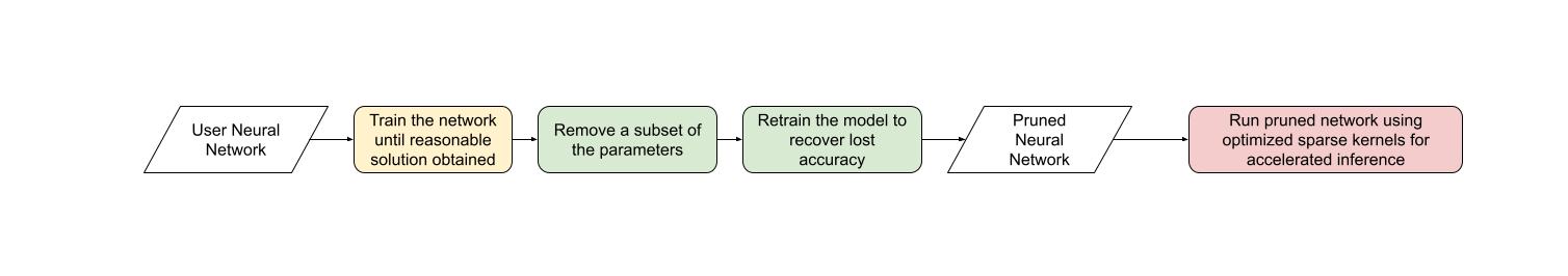
现在我们有了基线，是时候修剪 BERT 了。有很多不同的修剪策略，但其中最常见的一种是幅度修剪，它试图移除具有最低 L1 范数的权重。幅度修剪被 NVIDIA 在所有结果中使用，并且是一个常见的基线。

为了做到这一点，我们将使用 torch.ao.pruning 包，该包包含一个权重范数（幅度）稀疏化器。这些稀疏化器通过在模型的权重张量上应用掩码参数化来工作。这使得它们可以通过屏蔽被修剪的权重来模拟稀疏性。

我们还必须决定要应用稀疏性的模型层，在这个例子中是所有 nn.Linear 层，除了特定任务的输出头。这是因为半结构化稀疏性有形状约束，而特定任务的 nn.Linear 层不满足这些约束。

sparsifier = WeightNormSparsifier(
    # apply sparsity to all blocks
    sparsity_level=1.0,
    # shape of 4 elements is a block
    sparse_block_shape=(1, 4),
    # two zeros for every block of 4
    zeros_per_block=2
)

# add to config if ``nn.Linear`` and in the BERT model.
sparse_config = [
    {"tensor_fqn": f"{fqn}.weight"}
    for fqn, module in model.named_modules()
    if isinstance(module, nn.Linear) and "layer" in fqn
]

修剪模型的第一步是插入用于屏蔽模型权重的参数化。这是通过准备步骤完成的。每次我们尝试访问 .weight 时，我们都会得到 mask * weight 。

# Prepare the model, insert fake-sparsity parametrizations for training
sparsifier.prepare(model, sparse_config)
print(model.bert.encoder.layer[0].output)

然后，我们将执行一次单独的剪枝步骤。所有剪枝器都实现了一个 update_mask() 方法，该方法根据剪枝器的实现逻辑更新掩码。步骤方法调用 update_mask 函数，以稀疏配置中指定的权重为参数。

我们还将评估模型，以展示零样本剪枝（无需微调/重新训练）的精度下降。

sparsifier.step()
with torch.autocast("cuda"):
    with torch.no_grad():
        predictions = trainer.predict(tokenized_squad_dataset["validation"])
    pruned = compute_metrics(
        *predictions.predictions,
        tokenized_squad_dataset["validation"],
        squad_dataset["validation"],
    )
print("pruned eval metrics:", pruned)

在此状态下，我们可以开始微调模型，更新那些不会被剪枝的元素，以更好地补偿精度损失。一旦我们达到满意的状态，我们可以调用 squash_mask 来融合掩码和权重。这将移除参数化，我们最终得到一个零值的 2:4 密集模型。

trainer.train()
sparsifier.squash_mask()
torch.set_printoptions(edgeitems=4)
print(model.bert.encoder.layer[0].intermediate.dense.weight[:8, :8])

df["sparse_loss"] = pd.DataFrame(trainer.state.log_history)["loss"]
df.plot.line(x='step', y=["loss", "sparse_loss"], title="Loss vs. # steps", ylabel="loss")

加速 2:4 稀疏模型进行推理

现在我们有了这种格式的模型，我们可以像 QuickStart 指南中一样加速推理。

model = model.cuda().half()
# accelerate for sparsity
for fqn, module in model.named_modules():
    if isinstance(module, nn.Linear) and "layer" in fqn:
        module.weight = nn.Parameter(to_sparse_semi_structured(module.weight))

with torch.no_grad():
    predictions = trainer.predict(tokenized_squad_dataset["validation"])
start_logits, end_logits = predictions.predictions
metrics_sparse = compute_metrics(
    start_logits,
    end_logits,
    tokenized_squad_dataset["validation"],
    squad_dataset["validation"],
)
print("sparse eval metrics: ", metrics_sparse)
sparse_perf = measure_execution_time(
    model,
    batch_sizes,
    tokenized_squad_dataset["validation"],
)
print("sparse perf metrics: ", sparse_perf)

在进行幅度剪枝后重新训练我们的模型，几乎恢复了模型剪枝时丢失的所有 F1 分数。同时，我们实现了 1.28 倍的速度提升。请注意，并非所有形状都适合性能提升。当批量大小小且在计算稀疏内核上花费的时间有限时，它们可能比它们的密集对应物慢。

由于半结构化稀疏性被实现为张量子类，它与 torch.compile 兼容。当与 to_sparse_semi_structured 结合使用时，我们能够在 BERT 上实现总共 2 倍的速度提升。

指标	fp16	2:4 稀疏	delta / 加速	编译的
精确匹配（%）	78.53	78.44	-0.09
F1（%）	86.93	86.49	-0.44
时间（bs=4）	11.10	15.54	0.71 倍	否
时间（bs=16）	19.35	15.74	1.23 倍	否
时间（bs=64）	72.71	59.41	1.22 倍	否
时间（bs=256）	286.65	247.63	1.14 倍	否
时间（bs=4）	7.59	7.46	1.02 倍	是的
时间（bs=16）	11.47	9.68	1.18 倍	是的
时间（bs=64）	41.57	36.92	1.13 倍	是的
时间（bs=256）	159.22	142.23	1.12 倍	是的

结论 ¶

在本教程中，我们展示了如何剪枝 BERT 以实现 2:4 稀疏，以及如何加速 2:4 稀疏模型进行推理。通过利用我们的 SparseSemiStructuredTensor 子类，我们能够实现比 fp16 基线 1.3 倍的速度提升，并且通过 torch.compile 可以达到 2 倍。我们还展示了 2:4 稀疏的优势，通过微调 BERT 恢复任何丢失的 F1（86.92 密集型 vs 86.48 稀疏型）。