备注
点击此处下载完整示例代码
知识蒸馏教程 
创建于:2025 年 4 月 1 日 | 最后更新:2025 年 4 月 1 日 | 最后验证:2024 年 11 月 5 日
作者:亚历山德罗斯·查里顿
知识蒸馏是一种技术,它能够将大型、计算成本高的模型中的知识转移到较小的模型中,而不会丢失有效性。这使得在性能较弱的硬件上部署成为可能,从而使得评估更快、更高效。
在本教程中,我们将运行一系列实验,旨在提高轻量级神经网络的准确性,使用更强大的网络作为教师。轻量级网络的计算成本和速度将保持不变,我们的干预措施仅关注其权重,而不是其前向传递。这项技术的应用可以在无人机或移动电话等设备中找到。在本教程中,我们不使用任何外部包,因为我们需要的所有东西都在 torch 和 torchvision 中。
在本教程中,您将学习:
如何修改模型类以提取隐藏表示并用于进一步计算
如何修改 PyTorch 中的常规训练循环以包含额外的损失,例如在分类中添加交叉熵损失
如何通过使用更复杂的模型作为教师来提高轻量级模型的表现
前提条件 _
1 个 GPU,4GB 内存
PyTorch v2.0 或更高版本
CIFAR-10 数据集(由脚本下载并保存在名为
/data的目录中)
import torch
import torch.nn as nn
import torch.optim as optim
import torchvision.transforms as transforms
import torchvision.datasets as datasets

# Check if the current `accelerator <https://maskerprc.github.io/docs/stable/torch.html#accelerators>`__
# is available, and if not, use the CPU
device = torch.accelerator.current_accelerator().type if torch.accelerator.is_available() else "cpu"
print(f"Using {device} device")
加载 CIFAR-10 ...
CIFAR-10 是一个包含十个类别的流行图像数据集。我们的目标是预测每个输入图像的以下类别之一。
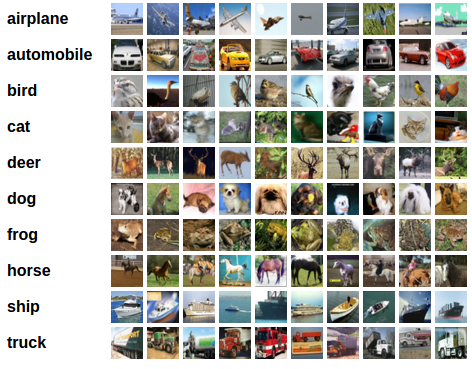
CIFAR-10 图像示例 
输入图像是 RGB 格式,因此它们有 3 个通道,大小为 32x32 像素。基本上,每张图像由 3 x 32 x 32 = 3072 个介于 0 到 255 之间的数字描述。在神经网络中,对输入进行归一化是一种常见做法,这有多种原因,包括避免常用激活函数的饱和以及提高数值稳定性。我们的归一化过程包括在每个通道上减去平均值并除以标准差。张量“mean=[0.485, 0.456, 0.406]”和“std=[0.229, 0.224, 0.225]”已经被计算出来,它们代表了预定义的 CIFAR-10 子集(旨在作为训练集)中每个通道的平均值和标准差。注意我们如何使用这些值来测试集,而不需要从头开始重新计算平均值和标准差。这是因为网络是在通过减去和除以上述数字产生的特征上训练的,我们希望保持一致性。此外,在现实生活中,我们无法计算测试集的平均值和标准差,因为根据我们的假设,这些数据在那个点将不可用。
作为总结,我们通常将这个预留集称为验证集,在优化模型在验证集上的性能后,我们使用另一个单独的集,称为测试集。这样做是为了避免根据单个指标的贪婪和有偏优化选择模型。
# Below we are preprocessing data for CIFAR-10. We use an arbitrary batch size of 128.
transforms_cifar = transforms.Compose([
    transforms.ToTensor(),
    transforms.Normalize(mean=[0.485, 0.456, 0.406], std=[0.229, 0.224, 0.225]),
])

# Loading the CIFAR-10 dataset:
train_dataset = datasets.CIFAR10(root='./data', train=True, download=True, transform=transforms_cifar)
test_dataset = datasets.CIFAR10(root='./data', train=False, download=True, transform=transforms_cifar)
备注
本节仅针对对快速结果感兴趣的 CPU 用户。只有在你对小型实验感兴趣时才使用此选项。请注意,使用任何 GPU,代码都应该运行得相当快。请仅选择训练/测试数据集的第一张 num_images_to_keep 图像。
#from torch.utils.data import Subset
#num_images_to_keep = 2000
#train_dataset = Subset(train_dataset, range(min(num_images_to_keep, 50_000)))
#test_dataset = Subset(test_dataset, range(min(num_images_to_keep, 10_000)))
#Dataloaders
train_loader = torch.utils.data.DataLoader(train_dataset, batch_size=128, shuffle=True, num_workers=2)
test_loader = torch.utils.data.DataLoader(test_dataset, batch_size=128, shuffle=False, num_workers=2)
定义模型类和实用函数
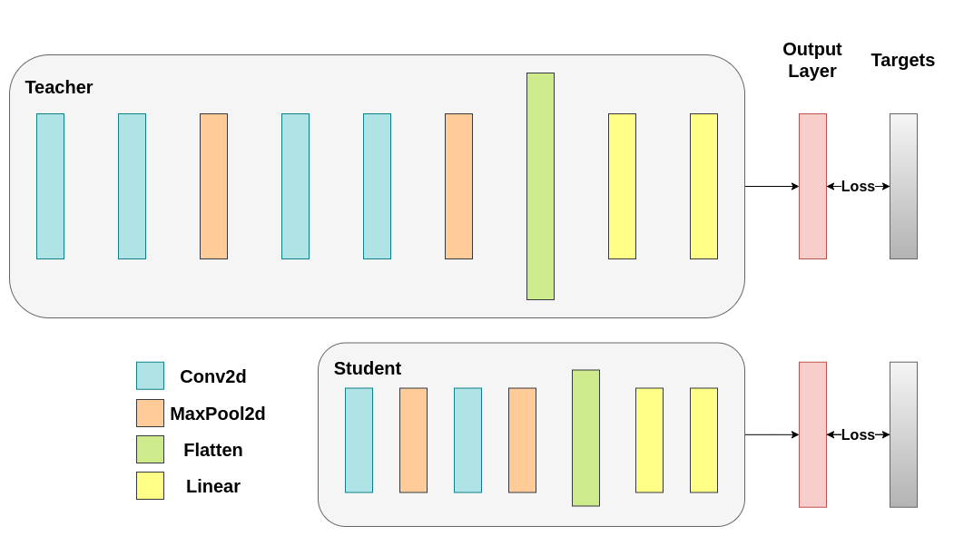
接下来,我们需要定义我们的模型类。在这里需要设置几个用户定义的参数。我们使用两种不同的架构,在实验中保持滤波器数量不变以确保公平比较。两种架构都是卷积神经网络(CNN),具有不同数量的卷积层作为特征提取器,随后是一个有 10 个类别的分类器。对于学生来说,滤波器和神经元的数量较小。
# Deeper neural network class to be used as teacher:
class DeepNN(nn.Module):
    def __init__(self, num_classes=10):
        super(DeepNN, self).__init__()
        self.features = nn.Sequential(
            nn.Conv2d(3, 128, kernel_size=3, padding=1),
            nn.ReLU(),
            nn.Conv2d(128, 64, kernel_size=3, padding=1),
            nn.ReLU(),
            nn.MaxPool2d(kernel_size=2, stride=2),
            nn.Conv2d(64, 64, kernel_size=3, padding=1),
            nn.ReLU(),
            nn.Conv2d(64, 32, kernel_size=3, padding=1),
            nn.ReLU(),
            nn.MaxPool2d(kernel_size=2, stride=2),
        )
        self.classifier = nn.Sequential(
            nn.Linear(2048, 512),
            nn.ReLU(),
            nn.Dropout(0.1),
            nn.Linear(512, num_classes)
        )

    def forward(self, x):
        x = self.features(x)
        x = torch.flatten(x, 1)
        x = self.classifier(x)
        return x

# Lightweight neural network class to be used as student:
class LightNN(nn.Module):
    def __init__(self, num_classes=10):
        super(LightNN, self).__init__()
        self.features = nn.Sequential(
            nn.Conv2d(3, 16, kernel_size=3, padding=1),
            nn.ReLU(),
            nn.MaxPool2d(kernel_size=2, stride=2),
            nn.Conv2d(16, 16, kernel_size=3, padding=1),
            nn.ReLU(),
            nn.MaxPool2d(kernel_size=2, stride=2),
        )
        self.classifier = nn.Sequential(
            nn.Linear(1024, 256),
            nn.ReLU(),
            nn.Dropout(0.1),
            nn.Linear(256, num_classes)
        )

    def forward(self, x):
        x = self.features(x)
        x = torch.flatten(x, 1)
        x = self.classifier(x)
        return x
我们使用了 2 个函数来帮助我们产生和评估我们原始分类任务的结果。其中一个函数被称作 train ,它接受以下参数:
model:通过此函数训练(更新其权重)的模型实例。train_loader:我们在上面定义了train_loader,其任务是向模型输入数据。epochs:我们循环遍历数据集的次数。学习率决定了我们向收敛方向迈出的步子大小。步子太大或太小都可能是有害的。
确定运行工作负载的设备。根据可用性,可以是 CPU 或 GPU。
我们的测试函数类似,但它将以 test_loader 调用以加载测试集的图像。
使用交叉熵训练两个网络。学生网络将作为基线:
def train(model, train_loader, epochs, learning_rate, device):
    criterion = nn.CrossEntropyLoss()
    optimizer = optim.Adam(model.parameters(), lr=learning_rate)

    model.train()

    for epoch in range(epochs):
        running_loss = 0.0
        for inputs, labels in train_loader:
            # inputs: A collection of batch_size images
            # labels: A vector of dimensionality batch_size with integers denoting class of each image
            inputs, labels = inputs.to(device), labels.to(device)

            optimizer.zero_grad()
            outputs = model(inputs)

            # outputs: Output of the network for the collection of images. A tensor of dimensionality batch_size x num_classes
            # labels: The actual labels of the images. Vector of dimensionality batch_size
            loss = criterion(outputs, labels)
            loss.backward()
            optimizer.step()

            running_loss += loss.item()

        print(f"Epoch {epoch+1}/{epochs}, Loss: {running_loss / len(train_loader)}")

def test(model, test_loader, device):
    model.to(device)
    model.eval()

    correct = 0
    total = 0

    with torch.no_grad():
        for inputs, labels in test_loader:
            inputs, labels = inputs.to(device), labels.to(device)

            outputs = model(inputs)
            _, predicted = torch.max(outputs.data, 1)

            total += labels.size(0)
            correct += (predicted == labels).sum().item()

    accuracy = 100 * correct / total
    print(f"Test Accuracy: {accuracy:.2f}%")
    return accuracy
交叉熵运行 
为了可重复性,我们需要设置 torch 的手动种子。我们使用不同的方法训练网络,因此为了公平比较,初始化网络以相同的权重是有意义的。首先使用交叉熵训练教师网络:
torch.manual_seed(42)
nn_deep = DeepNN(num_classes=10).to(device)
train(nn_deep, train_loader, epochs=10, learning_rate=0.001, device=device)
test_accuracy_deep = test(nn_deep, test_loader, device)

# Instantiate the lightweight network:
torch.manual_seed(42)
nn_light = LightNN(num_classes=10).to(device)
我们再实例化一个轻量级的网络模型来比较它们的性能。反向传播对权重初始化很敏感,因此我们需要确保这两个网络具有完全相同的初始化。
torch.manual_seed(42)
new_nn_light = LightNN(num_classes=10).to(device)
为了确保我们创建了第一个网络的副本,我们检查其第一层的范数。如果匹配,那么我们可以安全地得出结论,这两个网络确实是相同的。
# Print the norm of the first layer of the initial lightweight model
print("Norm of 1st layer of nn_light:", torch.norm(nn_light.features[0].weight).item())
# Print the norm of the first layer of the new lightweight model
print("Norm of 1st layer of new_nn_light:", torch.norm(new_nn_light.features[0].weight).item())
打印每个模型中的参数总数:
total_params_deep = "{:,}".format(sum(p.numel() for p in nn_deep.parameters()))
print(f"DeepNN parameters: {total_params_deep}")
total_params_light = "{:,}".format(sum(p.numel() for p in nn_light.parameters()))
print(f"LightNN parameters: {total_params_light}")
使用交叉熵损失训练和测试轻量级网络:
train(nn_light, train_loader, epochs=10, learning_rate=0.001, device=device)
test_accuracy_light_ce = test(nn_light, test_loader, device)
如我们所见,基于测试准确率,我们现在可以比较作为教师使用的更深网络和作为我们假设的学生使用的轻量级网络。到目前为止,我们的学生还没有干预教师,因此这种性能是由学生本身实现的。到目前为止的指标可以通过以下行查看:
print(f"Teacher accuracy: {test_accuracy_deep:.2f}%")
print(f"Student accuracy: {test_accuracy_light_ce:.2f}%")
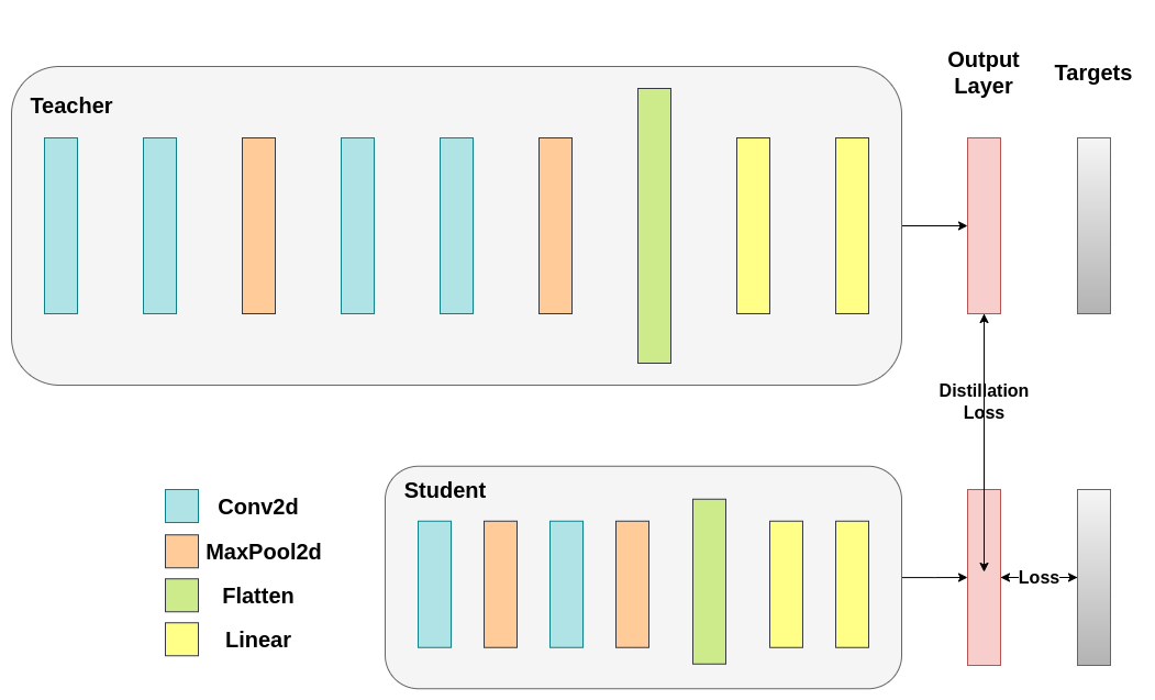
知识蒸馏运行 
现在让我们通过引入教师网络来提高学生网络的测试精度。知识蒸馏是一种简单的方法,基于两个网络都在我们的类别上输出一个概率分布的事实。因此,两个网络具有相同数量的输出神经元。该方法通过在传统的交叉熵损失中引入额外的损失来实现,该损失基于教师网络的 softmax 输出。假设一个训练良好的教师网络的输出激活包含学生网络在训练期间可以利用的额外信息。原始工作建议,利用软目标中小概率的比率可以帮助实现深度神经网络的潜在目标,即在数据上创建一个相似性结构,其中相似的对象被映射得更近。例如,在 CIFAR-10 中,如果一辆卡车的轮子出现,它可能会被误认为是汽车或飞机,但不太可能被误认为是狗。 因此,有理由假设,有价值的信息不仅存在于训练良好的模型的顶部预测中,还存在于整个输出分布中。然而,仅使用交叉熵并不能充分利用这些信息,因为非预测类别的激活通常非常小,传播的梯度不足以有意义地改变权重来构建这个理想的向量空间。
随着我们继续定义我们的第一个辅助函数,该函数引入了教师-学生动态,我们需要包含一些额外的参数:
T: 温度控制输出分布的平滑度。较大的T会导致更平滑的分布,因此较小的概率会得到更大的提升。soft_target_loss_weight: 分配给即将包含的额外目标的权重。跨熵的权重分配。调整这些权重将推动网络向优化某一目标发展。
知识蒸馏损失是从网络的 logits 计算得出的。它只返回梯度到学生端:
def train_knowledge_distillation(teacher, student, train_loader, epochs, learning_rate, T, soft_target_loss_weight, ce_loss_weight, device):
    ce_loss = nn.CrossEntropyLoss()
    optimizer = optim.Adam(student.parameters(), lr=learning_rate)

    teacher.eval()  # Teacher set to evaluation mode
    student.train() # Student to train mode

    for epoch in range(epochs):
        running_loss = 0.0
        for inputs, labels in train_loader:
            inputs, labels = inputs.to(device), labels.to(device)

            optimizer.zero_grad()

            # Forward pass with the teacher model - do not save gradients here as we do not change the teacher's weights
            with torch.no_grad():
                teacher_logits = teacher(inputs)

            # Forward pass with the student model
            student_logits = student(inputs)

            #Soften the student logits by applying softmax first and log() second
            soft_targets = nn.functional.softmax(teacher_logits / T, dim=-1)
            soft_prob = nn.functional.log_softmax(student_logits / T, dim=-1)

            # Calculate the soft targets loss. Scaled by T**2 as suggested by the authors of the paper "Distilling the knowledge in a neural network"
            soft_targets_loss = torch.sum(soft_targets * (soft_targets.log() - soft_prob)) / soft_prob.size()[0] * (T**2)

            # Calculate the true label loss
            label_loss = ce_loss(student_logits, labels)

            # Weighted sum of the two losses
            loss = soft_target_loss_weight * soft_targets_loss + ce_loss_weight * label_loss

            loss.backward()
            optimizer.step()

            running_loss += loss.item()

        print(f"Epoch {epoch+1}/{epochs}, Loss: {running_loss / len(train_loader)}")

# Apply ``train_knowledge_distillation`` with a temperature of 2. Arbitrarily set the weights to 0.75 for CE and 0.25 for distillation loss.
train_knowledge_distillation(teacher=nn_deep, student=new_nn_light, train_loader=train_loader, epochs=10, learning_rate=0.001, T=2, soft_target_loss_weight=0.25, ce_loss_weight=0.75, device=device)
test_accuracy_light_ce_and_kd = test(new_nn_light, test_loader, device)

# Compare the student test accuracy with and without the teacher, after distillation
print(f"Teacher accuracy: {test_accuracy_deep:.2f}%")
print(f"Student accuracy without teacher: {test_accuracy_light_ce:.2f}%")
print(f"Student accuracy with CE + KD: {test_accuracy_light_ce_and_kd:.2f}%")
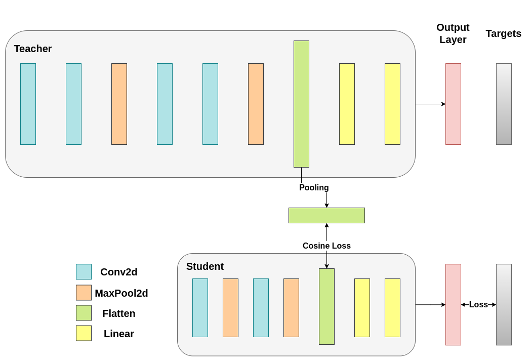
余弦损失最小化运行 
请随意调整控制 softmax 函数软度和损失系数的温度参数。在神经网络中,很容易将额外的损失函数添加到主要目标中,以实现更好的泛化等目标。让我们尝试为学生添加一个目标,但现在让我们关注他们的隐藏状态而不是输出层。我们的目标是通过对一个简单的损失函数进行最小化,将教师表示中的信息传递给学生,这意味着随后传递给分类器的展平向量随着损失减少而变得更加相似。当然,教师不会更新其权重,因此最小化仅取决于学生的权重。这种方法背后的原理是我们假设教师模型具有更好的内部表示,学生没有外部干预很难实现,因此我们人为地推动学生模仿教师的内部表示。 是否最终能帮助学生学习并不简单,因为推动轻量级网络达到这一点可能是一件好事,假设我们已经找到了一个导致测试精度更高的内部表示,但它也可能是有害的,因为网络有不同的架构,学生没有和教师一样的学习容量。换句话说,这两个向量,学生和教师的向量在各个分量上并不一定匹配。学生可能达到一个与教师不同的内部表示,这同样有效。尽管如此,我们仍然可以快速进行实验来了解这种方法的影响。我们将使用 CosineEmbeddingLoss ,其公式如下:
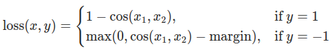
余弦嵌入损失公式
显然,我们首先需要解决一个问题。当我们对输出层应用蒸馏时,我们提到两个网络具有相同数量的神经元,等于类别的数量。然而,在经过我们的卷积层之后,情况并非如此。在这里,在最终卷积层展平之后,教师网络比学生网络有更多的神经元。我们的损失函数接受两个维度相同的向量作为输入,因此我们需要以某种方式使它们匹配。我们将通过在教师网络的卷积层之后包含一个平均池化层来解决这个问题,以将其维度降低以匹配学生网络的维度。
为了继续,我们将修改我们的模型类,或者创建新的类。现在,前向函数不仅返回网络的 logits,还返回卷积层之后的展平后的隐藏表示。我们为修改后的教师网络包含上述池化。
class ModifiedDeepNNCosine(nn.Module):
    def __init__(self, num_classes=10):
        super(ModifiedDeepNNCosine, self).__init__()
        self.features = nn.Sequential(
            nn.Conv2d(3, 128, kernel_size=3, padding=1),
            nn.ReLU(),
            nn.Conv2d(128, 64, kernel_size=3, padding=1),
            nn.ReLU(),
            nn.MaxPool2d(kernel_size=2, stride=2),
            nn.Conv2d(64, 64, kernel_size=3, padding=1),
            nn.ReLU(),
            nn.Conv2d(64, 32, kernel_size=3, padding=1),
            nn.ReLU(),
            nn.MaxPool2d(kernel_size=2, stride=2),
        )
        self.classifier = nn.Sequential(
            nn.Linear(2048, 512),
            nn.ReLU(),
            nn.Dropout(0.1),
            nn.Linear(512, num_classes)
        )

    def forward(self, x):
        x = self.features(x)
        flattened_conv_output = torch.flatten(x, 1)
        x = self.classifier(flattened_conv_output)
        flattened_conv_output_after_pooling = torch.nn.functional.avg_pool1d(flattened_conv_output, 2)
        return x, flattened_conv_output_after_pooling

# Create a similar student class where we return a tuple. We do not apply pooling after flattening.
class ModifiedLightNNCosine(nn.Module):
    def __init__(self, num_classes=10):
        super(ModifiedLightNNCosine, self).__init__()
        self.features = nn.Sequential(
            nn.Conv2d(3, 16, kernel_size=3, padding=1),
            nn.ReLU(),
            nn.MaxPool2d(kernel_size=2, stride=2),
            nn.Conv2d(16, 16, kernel_size=3, padding=1),
            nn.ReLU(),
            nn.MaxPool2d(kernel_size=2, stride=2),
        )
        self.classifier = nn.Sequential(
            nn.Linear(1024, 256),
            nn.ReLU(),
            nn.Dropout(0.1),
            nn.Linear(256, num_classes)
        )

    def forward(self, x):
        x = self.features(x)
        flattened_conv_output = torch.flatten(x, 1)
        x = self.classifier(flattened_conv_output)
        return x, flattened_conv_output

# We do not have to train the modified deep network from scratch of course, we just load its weights from the trained instance
modified_nn_deep = ModifiedDeepNNCosine(num_classes=10).to(device)
modified_nn_deep.load_state_dict(nn_deep.state_dict())

# Once again ensure the norm of the first layer is the same for both networks
print("Norm of 1st layer for deep_nn:", torch.norm(nn_deep.features[0].weight).item())
print("Norm of 1st layer for modified_deep_nn:", torch.norm(modified_nn_deep.features[0].weight).item())

# Initialize a modified lightweight network with the same seed as our other lightweight instances. This will be trained from scratch to examine the effectiveness of cosine loss minimization.
torch.manual_seed(42)
modified_nn_light = ModifiedLightNNCosine(num_classes=10).to(device)
print("Norm of 1st layer:", torch.norm(modified_nn_light.features[0].weight).item())
自然地,我们需要更改训练循环,因为现在模型返回一个元组 (logits, hidden_representation) 。使用一个样本输入张量,我们可以打印它们的形状。
# Create a sample input tensor
sample_input = torch.randn(128, 3, 32, 32).to(device) # Batch size: 128, Filters: 3, Image size: 32x32

# Pass the input through the student
logits, hidden_representation = modified_nn_light(sample_input)

# Print the shapes of the tensors
print("Student logits shape:", logits.shape) # batch_size x total_classes
print("Student hidden representation shape:", hidden_representation.shape) # batch_size x hidden_representation_size

# Pass the input through the teacher
logits, hidden_representation = modified_nn_deep(sample_input)

# Print the shapes of the tensors
print("Teacher logits shape:", logits.shape) # batch_size x total_classes
print("Teacher hidden representation shape:", hidden_representation.shape) # batch_size x hidden_representation_size
在我们的情况下, hidden_representation_size 是 1024 。这是学生最终卷积层的展平特征图,如您所见,它是其分类器的输入。对于教师来说也是 1024 ,因为我们通过 avg_pool1d 从 2048 中这样做。这里应用的损失只影响损失计算之前学生的权重。换句话说,它不影响学生的分类器。修改后的训练循环如下:
在余弦损失最小化中,我们希望通过返回梯度到学生来最大化两个表示之间的余弦相似度:
def train_cosine_loss(teacher, student, train_loader, epochs, learning_rate, hidden_rep_loss_weight, ce_loss_weight, device):
    ce_loss = nn.CrossEntropyLoss()
    cosine_loss = nn.CosineEmbeddingLoss()
    optimizer = optim.Adam(student.parameters(), lr=learning_rate)

    teacher.to(device)
    student.to(device)
    teacher.eval()  # Teacher set to evaluation mode
    student.train() # Student to train mode

    for epoch in range(epochs):
        running_loss = 0.0
        for inputs, labels in train_loader:
            inputs, labels = inputs.to(device), labels.to(device)

            optimizer.zero_grad()

            # Forward pass with the teacher model and keep only the hidden representation
            with torch.no_grad():
                _, teacher_hidden_representation = teacher(inputs)

            # Forward pass with the student model
            student_logits, student_hidden_representation = student(inputs)

            # Calculate the cosine loss. Target is a vector of ones. From the loss formula above we can see that is the case where loss minimization leads to cosine similarity increase.
            hidden_rep_loss = cosine_loss(student_hidden_representation, teacher_hidden_representation, target=torch.ones(inputs.size(0)).to(device))

            # Calculate the true label loss
            label_loss = ce_loss(student_logits, labels)

            # Weighted sum of the two losses
            loss = hidden_rep_loss_weight * hidden_rep_loss + ce_loss_weight * label_loss

            loss.backward()
            optimizer.step()

            running_loss += loss.item()

        print(f"Epoch {epoch+1}/{epochs}, Loss: {running_loss / len(train_loader)}")
我们需要修改我们的测试函数,出于同样的原因。在这里,我们忽略模型返回的隐藏表示。
def test_multiple_outputs(model, test_loader, device):
    model.to(device)
    model.eval()

    correct = 0
    total = 0

    with torch.no_grad():
        for inputs, labels in test_loader:
            inputs, labels = inputs.to(device), labels.to(device)

            outputs, _ = model(inputs) # Disregard the second tensor of the tuple
            _, predicted = torch.max(outputs.data, 1)

            total += labels.size(0)
            correct += (predicted == labels).sum().item()

    accuracy = 100 * correct / total
    print(f"Test Accuracy: {accuracy:.2f}%")
    return accuracy
在这种情况下,我们可以轻松地将知识蒸馏和余弦损失最小化包含在同一个函数中。在教师-学生范式下,结合方法以获得更好的性能是常见的。现在,我们可以运行一个简单的训练-测试会话。
# Train and test the lightweight network with cross entropy loss
train_cosine_loss(teacher=modified_nn_deep, student=modified_nn_light, train_loader=train_loader, epochs=10, learning_rate=0.001, hidden_rep_loss_weight=0.25, ce_loss_weight=0.75, device=device)
test_accuracy_light_ce_and_cosine_loss = test_multiple_outputs(modified_nn_light, test_loader, device)
中间回归器运行 
我们的朴素最小化由于多个原因不能保证更好的结果,其中一个原因是向量的维度。对于高维向量,余弦相似度通常比欧几里得距离更有效,但我们处理的是每个具有 1024 个分量的向量,因此提取有意义的相似性要困难得多。此外,正如我们提到的,推动教师和学生隐藏表示的匹配并不被理论支持。我们没有很好的理由去追求这些向量的 1:1 匹配。我们将通过包括一个额外的网络,称为回归器,来提供一个训练干预的最终示例。目标是首先提取教师卷积层后的特征图,然后提取学生卷积层后的特征图,最后尝试匹配这些图。然而,这一次,我们将在网络之间引入一个回归器以简化匹配过程。回归器将是可训练的,并且理想情况下会比我们朴素的最小化余弦损失方案做得更好。 它的主要任务是匹配这些特征图的维度,以便我们能够正确地定义教师和学生之间的损失函数。定义这样的损失函数提供了一个教学“路径”,这基本上是一个反向传播梯度的流程,这将改变学生的权重。针对我们原始网络中每个分类器之前的卷积层输出,我们有以下形状:
# Pass the sample input only from the convolutional feature extractor
convolutional_fe_output_student = nn_light.features(sample_input)
convolutional_fe_output_teacher = nn_deep.features(sample_input)

# Print their shapes
print("Student's feature extractor output shape: ", convolutional_fe_output_student.shape)
print("Teacher's feature extractor output shape: ", convolutional_fe_output_teacher.shape)
教师有 32 个过滤器,学生有 16 个过滤器。我们将包括一个可训练层,将学生的特征图转换为教师特征图的形状。在实践中,我们修改了轻量级类以返回中间回归器匹配卷积特征图大小后的隐藏状态,而将教师类修改为返回最终卷积层的输出,不进行池化或展平。
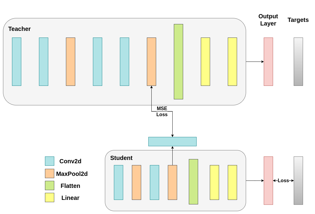
可训练层匹配中间张量的形状,均方误差(MSE)被正确定义:
class ModifiedDeepNNRegressor(nn.Module):
    def __init__(self, num_classes=10):
        super(ModifiedDeepNNRegressor, self).__init__()
        self.features = nn.Sequential(
            nn.Conv2d(3, 128, kernel_size=3, padding=1),
            nn.ReLU(),
            nn.Conv2d(128, 64, kernel_size=3, padding=1),
            nn.ReLU(),
            nn.MaxPool2d(kernel_size=2, stride=2),
            nn.Conv2d(64, 64, kernel_size=3, padding=1),
            nn.ReLU(),
            nn.Conv2d(64, 32, kernel_size=3, padding=1),
            nn.ReLU(),
            nn.MaxPool2d(kernel_size=2, stride=2),
        )
        self.classifier = nn.Sequential(
            nn.Linear(2048, 512),
            nn.ReLU(),
            nn.Dropout(0.1),
            nn.Linear(512, num_classes)
        )

    def forward(self, x):
        x = self.features(x)
        conv_feature_map = x
        x = torch.flatten(x, 1)
        x = self.classifier(x)
        return x, conv_feature_map

class ModifiedLightNNRegressor(nn.Module):
    def __init__(self, num_classes=10):
        super(ModifiedLightNNRegressor, self).__init__()
        self.features = nn.Sequential(
            nn.Conv2d(3, 16, kernel_size=3, padding=1),
            nn.ReLU(),
            nn.MaxPool2d(kernel_size=2, stride=2),
            nn.Conv2d(16, 16, kernel_size=3, padding=1),
            nn.ReLU(),
            nn.MaxPool2d(kernel_size=2, stride=2),
        )
        # Include an extra regressor (in our case linear)
        self.regressor = nn.Sequential(
            nn.Conv2d(16, 32, kernel_size=3, padding=1)
        )
        self.classifier = nn.Sequential(
            nn.Linear(1024, 256),
            nn.ReLU(),
            nn.Dropout(0.1),
            nn.Linear(256, num_classes)
        )

    def forward(self, x):
        x = self.features(x)
        regressor_output = self.regressor(x)
        x = torch.flatten(x, 1)
        x = self.classifier(x)
        return x, regressor_output
之后,我们再次更新我们的训练循环。这次,我们提取学生的回归器输出、教师的特征图,我们在这两个张量上计算 MSE (它们具有相同的形状,因此定义正确),并且基于这个损失进行反向传播梯度,除了分类任务的常规交叉熵损失之外。
def train_mse_loss(teacher, student, train_loader, epochs, learning_rate, feature_map_weight, ce_loss_weight, device):
    ce_loss = nn.CrossEntropyLoss()
    mse_loss = nn.MSELoss()
    optimizer = optim.Adam(student.parameters(), lr=learning_rate)

    teacher.to(device)
    student.to(device)
    teacher.eval()  # Teacher set to evaluation mode
    student.train() # Student to train mode

    for epoch in range(epochs):
        running_loss = 0.0
        for inputs, labels in train_loader:
            inputs, labels = inputs.to(device), labels.to(device)

            optimizer.zero_grad()

            # Again ignore teacher logits
            with torch.no_grad():
                _, teacher_feature_map = teacher(inputs)

            # Forward pass with the student model
            student_logits, regressor_feature_map = student(inputs)

            # Calculate the loss
            hidden_rep_loss = mse_loss(regressor_feature_map, teacher_feature_map)

            # Calculate the true label loss
            label_loss = ce_loss(student_logits, labels)

            # Weighted sum of the two losses
            loss = feature_map_weight * hidden_rep_loss + ce_loss_weight * label_loss

            loss.backward()
            optimizer.step()

            running_loss += loss.item()

        print(f"Epoch {epoch+1}/{epochs}, Loss: {running_loss / len(train_loader)}")

# Notice how our test function remains the same here with the one we used in our previous case. We only care about the actual outputs because we measure accuracy.

# Initialize a ModifiedLightNNRegressor
torch.manual_seed(42)
modified_nn_light_reg = ModifiedLightNNRegressor(num_classes=10).to(device)

# We do not have to train the modified deep network from scratch of course, we just load its weights from the trained instance
modified_nn_deep_reg = ModifiedDeepNNRegressor(num_classes=10).to(device)
modified_nn_deep_reg.load_state_dict(nn_deep.state_dict())

# Train and test once again
train_mse_loss(teacher=modified_nn_deep_reg, student=modified_nn_light_reg, train_loader=train_loader, epochs=10, learning_rate=0.001, feature_map_weight=0.25, ce_loss_weight=0.75, device=device)
test_accuracy_light_ce_and_mse_loss = test_multiple_outputs(modified_nn_light_reg, test_loader, device)
预计最终方法将比 CosineLoss 表现得更好,因为现在我们在教师和学生之间允许了一个可训练的层,这给学生提供了学习时的灵活性,而不是强迫学生复制教师的表示。包括额外的网络是基于提示的蒸馏背后的想法。
print(f"Teacher accuracy: {test_accuracy_deep:.2f}%")
print(f"Student accuracy without teacher: {test_accuracy_light_ce:.2f}%")
print(f"Student accuracy with CE + KD: {test_accuracy_light_ce_and_kd:.2f}%")
print(f"Student accuracy with CE + CosineLoss: {test_accuracy_light_ce_and_cosine_loss:.2f}%")
print(f"Student accuracy with CE + RegressorMSE: {test_accuracy_light_ce_and_mse_loss:.2f}%")
结论 
以上任何方法都不会增加网络的参数数量或推理时间,因此性能提升是以训练过程中计算梯度的微小代价为代价的。在机器学习应用中,我们主要关心推理时间,因为训练发生在模型部署之前。如果我们的轻量级模型仍然太重而无法部署,我们可以应用不同的想法,例如训练后量化。额外的损失可以在许多任务中应用,而不仅仅是分类,你可以尝试调整系数、温度或神经元数量等参数。在上述教程中,你可以随意调整任何数字,但请注意,如果你更改神经元/滤波器的数量,可能会出现形状不匹配的情况。
更多信息,请参阅:
脚本总运行时间:(0 分钟 0.000 秒)